Multilayer perceptrons (MLPs) represent the most prominent and well researched class of ANNs in classification, implementing a feedforward, supervised and hetero-associative paradigm [4, 36, 51]. MLPs consist of several layers of nodes , interconnected through weighted acyclic arcs from each preceding layer to the following, without lateral or feedback connections [4, 31, 32, 36]. Each node calculates a transformed weighted linear combination of its inputs of the form , with the vector of output activations from the preceding layer, the transposed column vector of weights , and a bounded non-decreasing non-linear function, such as the linear threshold or the sigmoid, with one of the weights acting as a trainable bias connected to a constant input [36]. Fig. 2 gives an example of a MLP with a [3-4-1] topology:

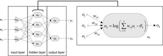
Fig. 2: Three layered MLP showing the information processing within a node, using a weighted sum as input function, the logistic function as sigmoid activation function and an identity output function.

For pattern classification, MLPs adapt the free parameter through supervised training to partition the input space through linear hyperplanes. To separate distinct classes, MLPs approximate a function of the form which partitions the X space into polyhedral sets or regions, each one being assigned to one out of the m classes of Y. Each node has an associated hyperplane to partition the input space into two half-spaces. The combination of the individual, linear node-hyperplanes in additional layers allows a stepwise separation of complex regions in the input space, generating a decision boundary to separate the different classes [36]. The orientation of the node hyperplanes is determined by the relative sizes of in including the threshold of a node , modelled as an adjustable weights to all nodes to offset the node hyperplane along for a distance from the origin to allow flexible separation. [30] The node non-linearity determines the output change as the distance from x to the node hyperplane. In comparison to threshold activation functions with a hard-limiting, binary class border, the hyperplanes associated with sigmoid nodes implement a smooth transition from 0 to 1 for the separation [23] allowing a graded response depending on the slope of the sigmoid function and the size of the weights. The desired output as a binary class membership is often coded with one output node or for multiple classification n nodes with respectively [23].

The representational capabilities of a MLP are determined by the range of mappings it may implement through weight variation. [36] Single layer perceptrons are capable of solving only linearly separable problems, correctly classifying data sets where the classes may be separated by one hyperplane [36]. MLPs with three layers are capable to approximate any desired bounded continuous function. The units in the first hidden layer generate hyperplanes to divide the input space in half-spaces. Units in the second hidden layer form convex regions as intersections of these hyperplanes. Output units form unisons of the convex regions into arbitrarily shaped, convex, non-convex or disjoint regions [1, 45]. Fig. 3 exemplifies this in a [2-6-2-1] network.

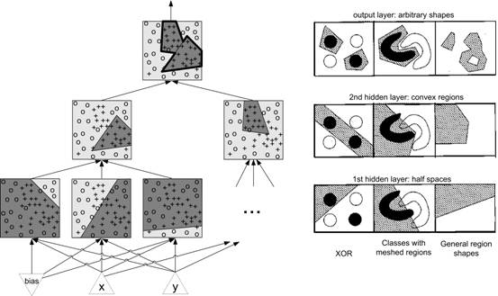
Fig. 3: Partitioning of the input space by linear threshold-nodes in an ANN with two hidden layers and one output node in the output layer and examples of separable decision regions [9]. For sigmoid activation functions smooth transitions instead of hard lined decision boundaries would be formed.

Given a sufficient number of hidden units, a MLP can approximate any complex decision boundary to divide the input space with arbitrary accuracy, producing a (0) when the input is in one region and an output of (1) in the other [28]. This property, known as a universal approximation capability, poses the essential problems of adequate model complexity in depth and size, i.e. the number of nodes and layers, and controlling the network training process to prevent overfitting. As perfect classification on training data does not necessitate generalisation for optimal separation of previously unseen data, simpler models with fewer parameters and training using early-stopping with out-of-sample evaluation on separate datasets are generally preferred. The network paradigm of MLP offers extensive degrees of freedom in modelling for classification tasks. Structuring the degrees of freedom, each expert must decide upon the static architectural properties P, the signal processing within nodes U, learning algorithm L and the pre-processed datasets D [15] in order to achieve the design goal, characterised through the objective function or error function O [22], calling for decisions upon ANN=[P, L, U, D, O]. The topology of the net is determined through the size NS and depth NL, of the network (number of layers, number of nodes in each hidden layer and coding of output vector through nodes in the output layer ), connectivity of the weight matrix K (fully or sparsely connected, shortcut connections etc.) and the activation strategy T (feedforward or with feedback): P=[NS, NL, K, T]. The signal processing within nodes, is determined by input function S (weighted sum or product, distance measures etc.), activation function A (tanh, logistic, sin, etc. with offsets, limits etc.) and output function F (linear, winner takes all variants or softmax), leading to U=[S,A,F]. Decisions concerning the learning algorithm encompass the choice of learning algorithm G (backpropagation, one of its derivatives, higher order methods or heuristics etc.), the complete vector of learning parameters for each individual layer and different phases in the learning process PTL, the procedure IP and number of initialisations for each network IN and the choice of the stopping method for the selection of the best network solution B. For classification, minimizing a squared error measure as the objective function O is inapplicable, as the goal is maximisation of correct classification. Consequently, the specification requires decisions upon MLP=[[NS, NL, K, T], [S, A, F], [G, PT, IP, IN, B], D, O], with the question of data pre-processing pre-determined for all competing methods in an early step of the knowledge discovery process.

Home | Neural Associations | Neural Applications | Neural Data Sources | Neural Community | Neural Contacts | Neural Publications | Neural News&Events | Neural Software | Neural Tutorials | Neural Links | Forecasting Principles

©  2002-2005 BI³S-lab - Hamburg, Germany - All rights reserved - Questions, Comments and Enquiries via eMail -  [Impressum & Disclaimer]
The Knowledge Portal on Forecasting with Neural Networks @ www.neural-forecasting.com -